"Pure Vernunft darf niemals siegen!"
- Tocotronic
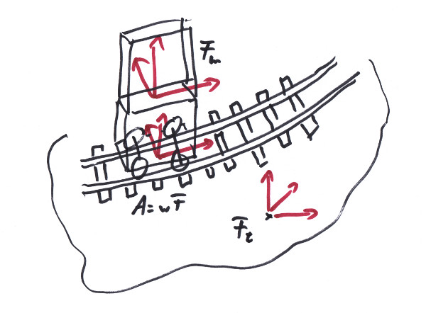
Moving along a track in a dynamic simulator can be done by defining special constraints for something we want to call a trackjoint. The trackjoint connects an anchor of a moving body with a track system that is fixed on another body [1]. Note that for now we do not simulate the axles or even the rotating wheels; our subject of consideration is the movement of a bogie as a whole. Also I want to stress, that at no point in this derivation (as in the whole of this book) we will transform to moving frames, because in general the velocities will not stay invariant in such frames. We are considering the things from the perspective of a resting global frame. With respect to that we maintain the following definitions:
    Time              t;       // simulation time.
    Time              dt;      // time step of one simulation cycle.
    Length            s;       // parameter along the track.
    Length            ds;      // distance the anchor moves along the track in a sim cycle.
    AnglePerLength    κ(s);    // curvature of the curve at track parameter s.
    AnglePerLength    τ(s);    // torsion of the curve at track parameter s.
    Angle             wt(s);   // twist of the track at track parameter s.

    Frame<Length,One> Fm(t);   // pose of the moving body's COM at simulation time t.
    Frame<Length,One> Ft(t);   // pose of the body's COM that holds the tracks at simulation time t.
    Frame<Length,One> F(s,t);  // point and orientation on the track at parameter s and at time t.
    Frame<Length,One> wF(s,t); // twisted frame F(s,t), rotatetd by wt(s).
    Frame<Length,One> A(t);    // anchor of the moving body; the point and the directions
                               // fixed on the body that are supposed to align with the track.

    Vector<Velocity>     vm; // Linear velocity of the moving bodie's COM.
    Vector<AnglePerTime> wm; // Rotation velocity of the moving bodie's COM moving along the track.
    Vector<Velocity>     vt; // Linear velocity of the track bodie's COM.
    Vector<AnglePerTime> wt; // Rotation velocity of the track bodie's COM.

    Matrix<3,6,One>    Jm; // matrix, specifying constraint of vm.
    Matrix<3,6,Length> Rm; // matrix, specifying constraint of wm.
    Matrix<3,6,One>    Jt; // matrix, specifying constraint of vt.
    Matrix<3,6,Length> Rt; // matrix, specifying constraint of wt.

    One erp               // 'error reduction parameter', see Chapter 6.
    Matrix<1,6,Length> e; // A 6 - dimensional vector, providing one number per
                          // constraint that describes the amount of positional error.
For the properties of a body look at Chapter 5; the curve geometry is explained in Chapter 3, that of a track in Chapter 4. Sometimes we talk about the moving body that carries the anchor: this does not mean, that the body that carries the tracks doesn't move; in general it does. As we've seen in Chapter 6, to define our trackjoint, we have to formulate the constraints in terms of the following equation:
Jm * vm + Rm * wm + Jt * vt + Rt * wt = erp/dt * e;
The above v and w refer to the movement of the centers of masses (COMs) of the bodies, from those we get the respective velocities of the anchor and the twisted frame as:
        Vector<Velocity> va = vm + wm % (A.P - Fm.P);
        Vector<AnglePerTime> wa = wm;
        Vector<Velocity> vp = vt + wt % (wF.P - Ft.P);
        Vector<AnglePerTime> wp = wt;
see Chapter 5. Each simulation step dt the values of the four matrices and e will get calculated by our trackjoint for the actual situation, then the engine will do a cycle of the algorithm, eventually fixing the velocities and moving the two bodies to their new positions accordingly. We now have to find a new position s + ds for our anchor along the track, meaning we need the ds.
The physics engine will have the relative movement of the two bodies along the tangent F.T(s,t) and not along the curve F.P(s,t), we take this relative movement as our;
ds = (A.P(t+dt) - A.P(t)) * F.T(s,t) - (F.P(s,t+dt) - F.P(s,t)) * F.T(s,t);
Note that we took the relative movement between the anchor's and the track's movement along F.T, since the track carrying body might move, too. Also note that we used F.P(s,t+dt) (as opposed to F.P(s+ds,t+dt)), since we want to subtract the movement of the old position on the track. We demand as a precondition that A(t) == F(s,t), which means that at t the anchor sat perfectly railed on the track at s. So we get;
ds = (A.P(t+dt) - F.P(s,t+dt)) * F.T(s,t);
There are some concerns about the fact that the simulation would not be perfect and how this would influence the validity of ds. But first, we will have some kind of error correction (see below) and above all secondly, this formular for ds has the advantage to immediately correct any aberrations along F.T: if A.P would for some reason get advanced along the curve, a greater ds would follow with the official track position; if F.P would be advanced, ds would move back. Any other choice would lead the F.P to advance or fall behind our A.P during the simulation and we would have to correct it.
With this ds, we find the new supposed pose of the anchor on the track, wF(s+ds,t+dt), but with a small margin of error, since our anchor was actually moved along the tangent and rotated according to the values at the start of ds. But note that we will do all movements and rotations according to the situation at s. So this is another second order error ( ~ds²) that will get corrected by our error correction.
Our obligation now is to calculate the J, R and e for our constraints.
Constraint 1, no relative movement along wF.N; on a track a linear movement sideways the track is prevented by the rails, so the relative movement in that direction would be zero. If there would be an aberration, a small correcting velocity will get introduced in the opposite direction;
(va - vp) * wF.N == erp/dt * -(A.P - wF.P) * wF.N;
The relative velocity on the left side is the velocity of the anchor as seen from the point on the track, an aberration of the anchor in positive wF.N direction has to lead to a compensating velocity in the opposite direction, hence the '-'. Substituting va, vp and using the relationship for the triple product (see Chapter 2), the left hand side becomes:
        ((vm + wm % (A.P - Fm.P)) - (vt + wt % (wF.P - Ft.P)) * wF.N ==
        wF.N * vm + ((A.P - Fm.P) % wF.N) * wm - wF.N * vt - ((wF.P - Ft.P) % wF.N) * wt;
from which we can take the element of the constraint equation as;
        Jm1   = wF.N;
        Rm1   = (A.P - Fm.P) % wF.N;
        Jt1   = -wF.N;
        Rt1   = wF.N % (wF.P - Ft.P);
        e1    = (wF.P - A.P) * wF.N;
        f1min = infinite;
        f1max = infinite;
Here the values represent the first row of the constraint equation and fmin will limit the maximum force applied in -wF.N direction and fmax be the maximum force applied in wF.N direction.
Constrain 2, no relative movement in -wF.B direction; the track supports the anchor by applying a force in the wF.B direction, but if anything would lift it, the constraint will offer no resistance. This plays quite similar to constraint 1;
(va - vp) * wF.B = erp/dt * -(A.P - wF.P) * wF.B;
yielding;
        Jm2 = wF.B;
        Rm2 = (A.P - Fm.P) % wF.B;
        Jt2 = -wF.B;
        Rt2 = wF.B % (wF.P - Ft.P);
        e2  = (wF.P - A.P) * wF.B;
        f2min= 0;
        f2max= infinite;
Constraint 3, a screwdriver rotation around wF.T according to torsion and twist; while the anchor is moving along the tangent direction it is supposed to follow the torsion of the curve τ(s) plus our twist wt(s).
wF.T * (wa - wp) - (τ(s) + dwt(s)/ds) * wF.T * (va - vp) == erp/dt * (A.T % wF.T + A.N % wF.N + A.B % wF.B) * wF.T;
If the curve's torsion would be zero and the twist would not change and we would have a perfect alignment of the N and B axes of the anchor and the twisted frame, the above equation would say that there'll be no relative rotation around wF.T. But since we have to rotate with the torsion and the changing twist as we move along the curve in wF.T direction, we have to subtract the second term to demand some specific amount of rotation. That the torsion computes into the equation like this can be seen from the Frenet/Serret equations (see Chapter 3): τ(s) specifies a rotation per length around T for the vectors N and B.
The right hand side demands a little rotation to correct the aberrations of the vectors A.N and A.B as far as the correcting rotation is along wF.T, of course. This is the idea: A and wF are supposed to be the same if the simulation would be perfect. If it aint, to bring A back to align with wF, little rotations are necessary. If they are small they can be simply added up. Since we are dealing with the rotation around wF.T here, only the part parallel to it can be used to correct the orientation of A. Note that the first term of the correctional rotation will cancel out. Substituting the velocities, we get from the left side;
wF.T * (wm - wt) - (τ(s) + dwt(s)/ds) * wF.T * ((vm + wm % (A.P - Fm.P) - (vt + wt % (wF.P - Ft.P));
which yields us;
        Jm3   = -(τ + dwt(s)/ds) * wF.T;
        Rm3   =  wF.T - (τ + dwt(s)/ds) * (A.P - Fm.P) % wF.T;
        Jt3   =  (τ + dwt(s)/ds) * wF.T;
        Rt3   = -wF.T + (τ + dwt(s)/ds) * (wF.P - Ft.P) % wF.T;
        e3    = (A.N % wF.N + A.B % wF.B) * wF.T;
        t3min = infinite;
        t3max = infinite;
The forces in this case actually become torques.
Constraint 4, no rotation around the normal direction; from Frenet/Serret equations you can see that there is no such rotation by the missing terms for dT/ds and dB/ds which would need some component in B or T direction respectively to rotate around N (see Chapter 3). Note that this relates to F.N and not to the twisted wF.N.
F.N * (wa - wp) == F.N * (wm - wt) == erp/dt * (A.T % wF.T + A.N % wF.N + A.B % wF.B) * F.N;
Still for error correction we would allow such a rotation along F.N, if it brings our anchor and the twisted frame closer together.
        Jm4   = 0;
        Rm4   = F.N;
        Jt4   = 0;
        Rt4   = -F.N;
        e4    = (A.T % wF.T + A.N % wF.N + A.B % wF.B) * F.N;
        t4min = infinite;
        t4max = infinite;
Constraint 5, proper rotation around F.B; from the Frenet/Serret equations (see Chapter 3), you see that the curvature κ(s) is the rotational change of F around F.B as you go along the curve, since the rotation of N and T around B would be;
        RNB = dN/ds - (dN/ds*B)*B = -κ*T;
        RTB = dT/ds - (dT/ds*B)*B = κ*N;
so we subtract the rotation caused by moving along the curve from the relative rotation between the bodies, and that should yield zero;
F.B * (wa - wp) - κ(s) * wF.T * (va - vp) == erp/dt * (A.T % wF.T + A.N % wF.N + A.B % wF.B) * F.B;
The left side is;
F.B * (wm - wt) - κ(s) * wF.T * ((vm + wm % (A.P - Fm.P)) - (vt+ wt % (wF.P - Ft.P));
So we get;
        Jm5 = - κ(s) * wF.T;
        Rm5 = F.B - κ(s) * (A.P - Fm.P) % wF.T;
        Jt5 =  κ(s) * wF.T;
        Rt5 = - F.B + κ(s)* (wF.P - Ft.P) % wF.T;
        e5  = (A.T % wF.T + A.N % wF.N + A.B % wF.B) * F.B;
        t5min = infinite;
        t5max = infinite;
Constraint 6, a motor for accelerating and braking; instead of applying forces to reach this goal, it is much more natural for a physics engine, to take a constraint. Since we deal with velocities, we have to specify a target velocity vTarget, that the engine would try to achieve by limited forces.
wF.T * (va - vp) == vTarget;
so the left side becomes;
wF.T * ((vm + wm % (A.P - Fm.P)) - (vt + wt % (wF.P - Ft.P));
this yields;
        Jm6 = wF.T;
        Rm6 = (A.P - Fm.P) % wF.T;
        Jt6 = -wF.T;
        Rt6 = wF.T % (wF.P - Ft.P);
        e6 = dt/erp * vTarget;
        f6min = motor_force_min;
        f6max = motor_force_max;
Note that the motor_force would be the total sum of a real motor's drive, a brake's force and the friction's force, all applied with propper signs.
With infinite constraint forces a bogie using this trackjoint would never derail. This can be overcome by monitoring the forces and torques and breaking the joint if they exceed certain limits. The problem with this approach is that in a railroad simulation - as with real railroads - one might have certain 'gaps' and 'kinks' inbetween the tracks. Even sudden changes in the curvature would lead to occasion hughe torques and thereby derailing. A better approach seems to be to limit the forces and torques to some reasonable values and then monitor the differences between A and wF. If these exceed some limits, then the trackjoint won't get applied in the simulation anymore, leaving the train to follow a ballistic trajectory.
This is how the trackjoint is implemented so far.
This trackjoint does not completely simulate the dynamic situation if it comes to a railroad bogie, since it does not take into account the spinning wheels that are sitting on two or more axles. This has several aspects: for one the missing inertia torques resulting from spinning masses (see Chapter 5), for second the rotating behaviour around F.N, which is possible together with an additional movement in wF.B direction and for third a gracefull tilting leading over to derailing. Last but not least the energy balance is not quite correct, since the spinning wheels would carry kinetic energy. Wether it is feasible to accurately simulate the rotational movements and thereby overcome these problems in a still stable simulation, or an approach that applies corrections to this basic trackjoint would do the trick - is still subject of research.
The units in the preceeding do not match exactly between the linear and the rotational constraints. I believe that has some deeper reason. But I have to investigate this further: after all for a single constraint in theory it does not matter to multiply both sides of the equation by a number - maybe even Length{1}. Probably the rotational equations have to get multiplied by a Length, where the actual value will make the negotiaton factor about how important it is to get a rotation right vs. to get the linear position right. In that case it would be some LengthPerAngle value, describing what would be a comparable severe linear failure to some given angular failure ...
There is a contradiction with our prerequisites when we constructed the motor. In Chapter 6 we assumed at one point that the constraint forces would do no work in total, while the motor in obtaining a target velocity clearly does that. It adds energy to the system. Nevertheless experience with ODE and NVidia PhysX shows that a stable simulation is gained by doing that anyway. It stays subject of research, wether we can relax the prerequisite somehow. In the meantime we resort to the fact, that we introduced the target velocity on the right side of the equation, being an error correction term in fact. These error corrections - if violated - clearly add (or remove) energy to the system, but they were introduced additionally. Find comfort in the phrase "Pure Vernunft darf niemals siegen (Pure reason must never win)" - it works for me at least.