"Und wir tanzen auf dem Staub unserer Helden"
-Sondaschule
A joint is a connection between two rigid bodies or a rigid body and the static or kinematic environment, which limits their relative movement to some extent. An example would be a hinge joint that connects a door to a static wall or a bogie to a waggon. Another example can be a slider like connection, that allows a linear relative movement between two bodies, but restricts all relative rotations and the other two directions of relative linear movement. We are thinking here in terms of degrees of freedom (DOFs) that a system of n bodies has. In three dimensional space one unconfined rigid body can move in three directions, while it might rotate around an axis at the same moment. The direction of the axis gives the orientation of the rotation, its length the angular velocity; hence we have another three DOFs, making up 6 DOFs in total for one body. If we tie the body with a hinge like a door to a wall, all of the sudden, there is only one degree of freedom left. This is the turning angle around the hinge, when we open or close that door. So a hinge joint removes 5 DOFs from the body.
If we have n bodies in a system that are not connected by joints whatsoever, the DOFs of the single bodies add up to 6*n DOFs for the system in total. For example, if we connect a bogie to a waggon base by a hinge, there are l = 6*2 - 5 == 7 DOFs left for the system. These are 6 DOFs for the system to move and rotate as a whole plus the one hinge angle. A joint can remove any number of DOFs from a system (up to the total number of DOFs in the system, of course); e.g. a joint that restricts a bodies COM to some plane, but let it rotate freely would remove only one DOF from the system. We call this a constraint. So a joint might have a number m of constraints, depending of how many DOFs it removes from the system. For our hinge joint, m is 5.
How can we guarantee such a hinge joint condition in a system of rigid bodies governed by the laws or Sir Newton's dynamics? Well, in Chapter 5 we already ranted about the tautology of that method: whenever we see a body moving in some particular way, we just assume that there will be forces acting that way. We call them constraint forces fc or constraint torques Tc respectively. Actually we already used this line of thinking in Chapter5, when we removed all degrees of freedom that the single points of mass had, except of six, to build a rigid body. We did this by assuming internal forces that are just right to accomplish that feat. Let us first describe a joint between a body and its static environment in terms of the velocities [1]:
J*v + R*w == 0;
here J and R are 3 x m dimensionated matrices that will restrict the velocities in some way. For example to restrict the body to move in a plane parallel to the x/y plane, we would pick a joint with one constraint:
J = ( 0, 0, 1 ); R = ( 0, 0, 0 );
which would give vz == 0. This kind of definition allows also a description of the constraints for the accelerations (by its first derivative) which would be closely connected to our wanted constraint forces as we will see. To restrict a body to an arbitrary plane with normal vector a = { ax, ay, az }, we would pick:
J = ( ax, ay, az ); R = ( 0, 0, 0 );
which would give: a * v == 0, meaning no movement in direction 'a'. Note that to restrict the body to a specific plane that starting point of the body is significant; from the plane it once is on it can not escape during the simulation as long as the constraint holds. To restrict the movement to a line two perpendicular vectors a, b would be needed and two constraints for the joint:
        J = ( ax,  ay,  az )  R = ( 0, 0, 0 )
            ( bx,  by,  bz );     ( 0, 0, 0 );
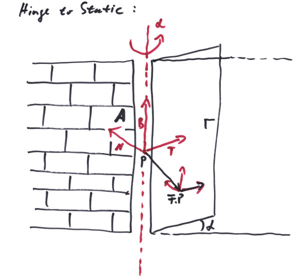
which would give the two equations a * v = 0 and b * v = 0, so v can only point in direction c = a % b. Note that while traveling freely into direction c, the body also is able to rotate around what axis soever. A hinge for a door can be described by an anchor Frame<Length,One> A, which gives a point A.P along the hinge axis as well as the axis direction with A.B. For the body with frame F and D = F.P - A.P we can build:
            (      0,      0,      0 )           ( A.T.dx, A.T.dy, A.T.dz )
            (      0,      0,      0 )           ( A.N.dx, A.N.dy, A.N.dz )
      J =   ( A.B.dx, A.B.dy, A.B.dz );      R = (      0,      0,      0 );
            (   D.dx,   D.dy,   D.dz )           (      0,      0,      0 )
            (         A.B % D        )           (       -A.B * D²        )
where we wrote the vector components with the exception of the last constraint where it was to laborious for us. The first and second constraints forbid any rotational velocities around A.T and A.N, so that the body only can rotate around A.T % A.N == A.B. This is along the same line of thinking as with the restriction of linear movement along some axis. The third constraint then says that the body can not move in the direction of the rotational axis. The fourth constraint guaranties that the distance of the body to the axis stays constant, while the last constraint puts the linear and angular movement in a relationship, saying that:
        (A.B % D) * v - A.B * D² * w == 0
        A.B % D * dr/dt == A.B * D² * dα/dt
        A.B % D/|D| * dr == A.B * |D| * dα
This is the tangential movement of the rotation dr equals the rotation dα around A.B. Note that with D the J, R might become time dependent, so in the simulation the constraints have to be evaluated each simulation step anew.
A joint between two bodies i and j will be formulated like this [1]:
Ji*vi + Ri*wi + Jj*vj + Rj*wj == 0
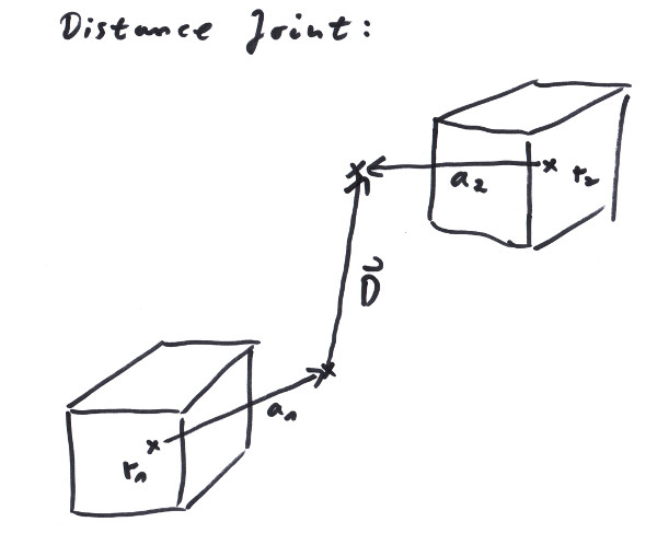
Here Ji, Ri, Jj, Rj, are 3 x m dimensionated matrices that will tie the velocities of the two bodies to each other. For example, a distance joint that might get used to couple two waggons together would maintain the distance between two fixpoints on the two bodies, but will not restrict the positions and orientations of the two bodies otherwise. With r1, r2 being the centers of mass and a1, a2 being positional anchors:
        Position<Length> r1, r2;
        Vector<Length> a1, a2;
        Vector<Length> D = (r1 + a1) - (r2 + a2);

        D * dD/dt                                       == 0; // the relative velocity in the direction of the connection has to be 0.
        D * ((v1 + da1/dt) - (v2 + da2/dt))             == 0;
        D * ((v1 + w1 % a1) - (v2 + w2 % a2))           == 0; // the |a| are constant, so da/dt = w % a are pure rotations.
        D * v1 + D * (w1 % a1) - D * v2 - D * (w2 % a2) == 0;
        D * v1 + (a1 % D) * w1 - D * v2 - (a2 % D) * w1 == 0; // using the relations for the triple product, see Chapter 3.

        ->  J1 = ( D ); R1 = ( a1 % D ); J2 = ( -D ); R2 = ( D % a2 );
One body and two body contraints we talked so far; theoretically we might have n body contraints with the extended formular:
∑ (Ji*vi + Ri*wi) == 0; // for i = 0 -> n
Our joints for a single body or two bodies would fit into that scheme by making all the other Ji, Ri null. Common physics engines like ODE or Nvidia PhysX don't use such multi body constraints. One reason is their rare practical use, the other is the better performace that can be achieved by restricting the joints [2]. In the next section we will take a look at what common physics engines actually calculate. For such a kind of general discussion it is usefull to formulate the parameters as one giant vector q with 6*n dimensions, containing all linear and all angular parameters for all the bodies in the n - body system. The constraints then become a single matrix J of dimensions 6n x m and the constraint equation becomes:
J * dq == 0;
Our algorithm from Chapter 5 would now look like that:
Step 3 and step 4 are not exactly independend, since we need the dynamic equations to figure out what the constraint forces would be. From Chapter 5 we remember:
        m * dv/dt == fe + fc;
        I * dw/dt == Te + Tc - w % L;
Note that I splitted the forces and the torques into their external parts (e) and another part (c) that represents the forces and torques that we will introduce to maintain our constraints. Actually, since w and L are known values, we like to subsume these inertia caused torque into the Te value (actually it looks like physics engines tend to omit this 'fun-factor' completely - as if reality could be improved -, but we can easily reintroduce it as an external torque). This makes the two equations rather uniform looking. We could drive this even further to yield one six dimensional vector equation for all six degrees of freedom of the rigid body. We don't want to do this in detail, since we'll use a physics engine for all those heavy calculations, but we do want to understand how in principal the calculation of fc and Tc is done.
We now jump high and pluck the apple; the physics engines do the following [2, 3]: they put the first two equations (each being 3 equations actually) - that relate to one body - into one giant 6*n dimensional vector equation that contains the state q (all linear and angular parameters of all the bodies, 6n dimensions) of the whole system and yield:
M * d²q/dt² = Qe + Qc;
With M being an 6n x 6n inertia matrix, containing the masses and the inertia tensors of all the bodies in or close around the diagonal with all the other elements being zero. This is called a sparse banded matrix, which as such offers efficient methods for numerical solving. The Qs are 6n dimensionated vectors that hold all the forces and torques for all the bodies.
The equations for all the constraints are also contracted into a single constraint equation (see above):
J * dq/dt == 0;
With an 6n x m dimensional matrix J, where m is the total number of contraints and dq/dt are the velocities of the q.
Now comes some rather reasonable idea: all the constraint forces Qc in total should do no work, which is the product of the force and the displacement in the direction of the force. This means, the constraint forces can not add or remove energy from our system of constrained bodies. It writes as a single equation:
        Qc * dq == 0;
        -> (M * d²q/dt² - Qe) * dq == 0;
if - and this is important - we choose dq as a variation of our parameters in a way so the constraints are respected:
J * dq == 0;
This means the displacement is one of the ones that really can happen; for the others we do not care. Note that we do not demand that there might be some single dq for which the relationship holds, but we demand that for all dq that respect J * dq == 0, the (M * d²q/dt² - Qe) * dq == 0 relationship holds.
And here comes some rather surprising idea: just let us make a vector λ of dimension m, with all the λ1, λ2, etc components being completely unknown and multiply the constraint equation by it:
        λ * (J * dq) == 0;
       -> (Transposed(J) * λ) * dq == 0;
Nobody can stop us from doing that, not even from subtracting this equation from the first one that describes the work as being zero:
(M * d²q/dt² - Qe - Transposed(J) * λ) * dq == 0;
These are two 6n dimensional vectors scalar multiplicated by each other. From this we want to follow that the first one is zero, namely:
M * d²q/dt² - Qe - Transposed(J) * λ == 0;
This is how it works: the dq we can pick freely with the restriction that they still have to fulfill the constraints equations. So from the 6n values in dq we can only choose 6n-m by free choice, the rest then would be set. But we have m λs. So let us pretend we calculate the m λs in a way that the first m components of the vector actually get zero (there might be some dqi that are set independent from the others, typically by dqi == 0, these we would bring gracefully to the top by reordering the parameters). This means, we don't have to care about the first m dqs, since they get multiplied by zero anyway. The rest we can pitch as we want, or differently said: the first m equations equal 0 for all dq we can possibly pick. So just be evil: pick all of the 6n-m dq to be zero with the exception of one. It's counterpart hence has to be zero. And since the equation has to hold not only for one but for all possible dq, we can do this for all the remaining components [4].
Admittedly, this is an amazing argument. If we put the result a little bit in shape:
M * d²q/dt² == Qe + Transposed(J) * λ;
we see by comparison with the dynamics equation, that:
Qc = Transposed(J) * λ;
Now we are close: the constraint equation can be derived for the time:
dJ/dt * dq/dt + J * d²q/dt² == 0
The acceleration is:
        d²q/dt² == Inverse(M) * (Qe + Transposed(J) * λ);

        -> dJ/dt * dq/dt + J * Inverse(M) * (Qe + Transposed(J) * λ) == 0;
        J * Inverse(M) * Transposed(J) * λ == -dJ/dt * dq/dt -  J * Inverse(M) * Qe;
                      A                * λ ==                b;
For this kind of matrix equation with known A and b the λs can get calculated by numerical methods fast [2]. The derivative of J can be gotten from the change since the last simulation steps. Then the λ is used to calculate the accelerations and from that the velocities and positions can get updated.
With the calculation of the λs in step 3 of the algorithm, a physics engine has access to the actual constraint forces. Typically the user is able to do a query for the forces used in a simulation step. This can be used e.g. for making joints breakable. A distance joint that simulates a coupling between two waggons might be removed by the user if the forces become stronger then some limit within one or more simulation cycles. That would simulate breaking couplings in a train.
Limiting the constraint forces is another application. After calculating Qc = Transposed(J) * λ; for some Qcmin, Qcmax, the forces can be clipped prior to doing step 4. For example contact joints that are used to simulate collisions between bodies are built with Qcmin = 0, Qcmax = +infinite to forbid a movement against a normal vector in order to avoid penetration of the two bodies. But the constraint forces are limited at one side to zero, so the bodies can freely move apart, while all forces that push them together are balanced by a constraint force, no matter how strong they get. Note that all force limits that are not 0 or +-infinite or that are not immediately released as soon as some movement in their direction happens, might violate our prerequisite of constraint forces of not adding or removing energy from the system. These cases might lead to non realistic effects.
A motor is a situation where we intentionally want to add energy to a system. It would be possible to simulate a motor by adding external forces or torques to the system, but especially if large forces or torques are involved, this might lead to instabilities. A better and more stable approach is to formulate a constraint, where the right side of the constraint equation is not zero anymore:
J * dq/dt == c;
For example, the movement along a line, defined by 'a', might be constrained by:
        Vector<One> a = Ex<One>;
        Velocity c = 2_mIs;

        ( a.dx, a.dy, a.dz ) * v == c;
This would force the velocity along 'a' of a body to be c. It would bring the body to that velocity in one simulation step. But with limits for the constraint forces to values that can actually be applied by a motor according to its throttle setting, it becomes realistic. Brakes and friction can be simulated the same way by setting c to zero, but limiting the constraint forces to the braking and/or friction forces. Propulsion, brake and friction forces can all get accumulated within one joint.
In a perfect world we would constrain the velocities and if the joints would be satisfied by the initial parameters of the system (e.g. a body restricted to some plane would initially sit on that plane), then according to the allowed velocities the joint can not be violated later. In reality the initial parameters might not match the constraints exactly; furthermore numerical calculations introduce errors that tend to grow over time. A good correction mechanism to meet this is to make c a velocity that corrects the positional errors. For example:
        VectorBundle<Length,One> A{ Origin3D<Length>, Ex<One> };
        One erp = 0.5f;
        Velocity c = -erp * (F.P - A.P) * A.T / dt;

        ( A.T.dx, A.T.dy, A.T.dz ) * v = c
That c now measures the distance of the body to the plane and constructs a velocity based on the time step dt that would move the body back into the plane in one simulation step, provided that e == 1. This e is the 'error reduction parameter'. It offers the possibility to switch off error correction completely (e == 0); since a sudden change in position might not look realistic and can even collide with internal optimisations of the physics engine, normally it is better to use a smaller e, so the error will be corrected slowly over several simulation cycles. Note that as long as there is no positional error, c would evaluate as 0.